Introduction
One of the main responsibilities of teachers and professors in the humanities is grading students essays [1]. Of course, manual essay grading for a classroom of students is a time-consuming process, and can even become tedious at times. Furthermore, essay grading can be plagued by inconsistencies in determining what a “good” essay really is. Indeed, the grading of essays is often a topic of controversy, due to its intrinsic subjectivity. Instructors might be more inclined to better reward essays with a particular voice or writing style, or even a specific position on the essay prompt.
With these and other issues taken into consideration, the problem of essay grading is clearly a field ripe for a more systematic, unbiased method of rating written work. There has been much research into creating AI agents, ultimately based on statistical models, that can automatically grade essays and therefore reduce or even eliminate the potential for bias. Such a model would take typical features of strong essays into account, analyzing each essay for the existence of these features.
In this project, which stems from an existing Kaggle competition sponsored by the William and Flora Hewlett Foundation [2], we have attempted to provide an efficient, automated solution to essay grading, thereby eliminating grader bias, as well as expediting a tedious and time-consuming job. While superior auto-graders that have resulted from years of extensive research surely exist, we feel that our final project demonstrates our ability to apply the data science process learned in this course to a complex, real-world problem.
Data Exploration
It was unnecessary for us to collect any data, as the essays were provided by the Hewlett Foundation. The data is comprised of eight separate essay sets, consisting of a training set of 12,976 essays and a validation set of 4,218 essays. Each essay set had a unique topic and scoring system, which certainly complicated fitting a model, given the diverse data. On the bright side, the essay sets were complete—that is, there was no missing data. Furthermore, the data was clearly laid out in both txt and csv formats that made importing them into a Pandas DataFrame a relatively simple process. In fact, the only complication to arise from collecting the data was a rather sneaky one, only discovered in the later stages when we attempted to spell check the essays. A very small number of essays contained special characters that could not be processed in unicode (the most popular method of text encoding for English). To handle these special characters, we used ISO-8859-1 text encoding, which eliminated encoding-related errors.
The training and validation sets did have plenty of information that we deemed to be extraneous to the scope of our project. For example, the score was often broken down by scorer, and at times into subcategories. We decided to take the average of the overall provided scores as our notion of “score” for each essay. Ultimately, then, the three crucial pieces of information were the essay, the essay set to which it belonged, and the overall essay score.
With the information we needed in place, we tested a few essay features at a basic level to get a better grasp on the data’s format as well as to investigate the sorts of features that might prove useful in predicting an essay’s score. In particular, we calculated the number of words and the vocabulary sizes (number of unique words), for each essay in the training set, plotting them against the provided essay scores.
We hypothesized that word count would certainly be correlated positively with essay score. As students, we note that longer essays often reflect deeper thought and stronger content. On the flip side, there is also value in being succinct by eliminating “filler” content and unnecessary details in papers. As such, we figured that the strength of correlation would weaken as the length of the essays increased.
With regard to vocabulary sizes, we reasoned that individuals who typically read and write more have broader lexicons, and as such a larger vocabulary size would correlate with a higher quality essay, and thus a higher score. After all, the more individuals read and write, the greater their exposure to a larger vocabulary and a more thorough understanding of how properly use it in their own writing. As such, a skilled writer will likely use a variety of exciting words in an effort to more effectively keep readers engaged and to best express their ideas in response to the prompt. Therefore, we hypothesized that a larger vocabulary list would correlate with a higher essay score.
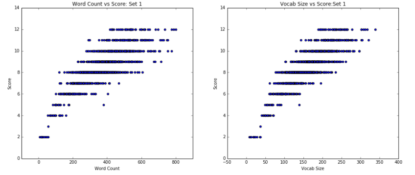
The first notable finding, as evidenced in Figure 1, is that the Word Count vs. Score scatter plots closely mirror the Vocab Size vs Score scatter plots when paired by essay set. This suggests that there might be a relationship between the length of the essay and the different number of words that a writer uses, a discovery that makes sense: a longer essay is bound to have more unique words.
From the Word Counts vs Score scatter plots, we note that in general, there seems to be an upward, positive trend between the essay words counts and the score, with the data expanding in a funnel-like shape. In set 4, there are certainly a couple of essays with the score of 1 that have a smaller word count and vocabulary list than the essays with a score of 0, but that result is likely due to essays with a score of 0 being either incomplete or unrelated to the prompt. As such, these data represent outliers and therefore do not speak to the general, positive relationship. Similar trends and patterns hold true for Vocab Size vs Score.
For set 3, we see that as the scores increase, the range of values for the number of words increases, meaning the number of words themselves tend to increase with score in a tornado-like shape, as mentioned. That is, while low scores were almost exclusively reserved for short essays, good grades were assigned to essays anywhere along the word count spectrum. In other words, there are many essays which have comparable word and vocabulary counts with different scores—especially those of smaller size. On the other hand, those essays with a distinctly greater word count and vocabulary size clearly receive higher scores. Similarly, for sets 1, 2, 4, 5, 6, and 7, we noted that, although the average word count increases as the score increases, the range of word counts also becomes wider, resulting in significant overlap of word counts across scores. This reinforces the conclusion that while word count is, in fact, correlated to essay score, the correlation is weaker for higher-scored essays, since there exists a significant overlap of word count across different scores.
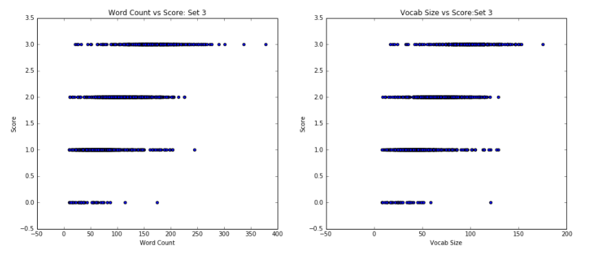
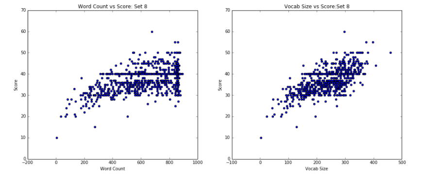
Essay set 8 has different trends: essays with large word counts and vocabulary sizes range greatly in scores. However, despite the unpredictability highlighted by this wide range, a clear predictor does emerge: essays with a small word count and small vocabulary size are graded with correspondingly low scores. As such, unlike in other datasets, where higher word and vocabulary counts equate to higher scores, we see that higher word essays may still be graded across the full range of scores. On the other hand, low word and vocabulary counts are a strong predictor of low score. In our investigation of this phenomenon, we noticed a disparity with essay set 8: it was the only prompt that has a maximum essay length, as measured by word count. Ultimately, this factor could have encouraged essays of particular size, regardless of essay quality.
The Baseline
With a sufficient grasp on the data, we set out to create a baseline essay grading model to which we could compare our final (hopefully more advanced) model. In order to generalize the model across different essay sets (which each contained different scoring systems, as mentioned), we standardized each essay set’s score distribution to have a mean of 0 and a standard deviation of 1.
For the baseline model, we began by considering the various essay features in order to choose the ones that we believed would be most effective, ultimately settling on n-grams. In natural language processing, n-grams are a very powerful resource. An n-gram refers to a consecutive sequence of n words in a given text. As an example, the n-grams with n=1 (unigram) of the sentence “I like ice cream” would be “I”, “like”, “ice”, and “cream”. The bigrams (n=2) of this same sentence would thus be “I like”, “like ice”, and “ice cream”. Ultimately, for a sufficiently large text, n-grams may be analyzed for any positive, nonzero integer n.
In analyzing a text, using n-grams of different n values may be important. For example, while the meaning of “bad” is successfully conveyed as a unigram, it would be lost in “not good,” since the two words would be analyzed independently. In this scenario, then, a bigram would be more useful. By a similar argument, a bigram may be effective for “not good,” but less so for “bad,” since it could associate the word with potentially unrelated words. For our baseline, however, we decided to proceed with unigrams in the name of simplicity.
To quantify the concept of n-grams, we used an information retrieval method called term frequency-inverse document frequency (tf-idf). This measure quantifies the number of times that an n-gram appears in the essay while weighting them based on how frequently the words appear in a general corpus of text. In other words, the tf-idf measure provides a powerful way of standardizing n-gram counts based on the expected number of times that they would have appeared in an essay in the first place. As a result, while the count of a particular n-gram may be large if found often in the text, this can be offset when processed by the tf-idf method if the n-gram is one already frequently appears in essays.
As such, given the benefits of n-grams and their quantification via the tf-idf method, we created a baseline model using unigrams with tf-idf as the predictive features. As our baseline model, we decided to use a simple linear regression model to predict a set of (standardized) scores for our training essays.
To evaluate our linear regression model, we opted to eschew the traditional R^2 measure in favor of Spearman’s Rank Correlation Coefficient. While the traditional R^2 measures determines the accuracy of our model—that is, how closely the predicted scores correspond to the true scores—Spearman instead measures the strength and direction of monotonic association between the essay feature and the score. In other words, it determines how well the ranking of the features corresponds with the ranking of the scores. The benefit of this approach is that this is a useful measure for grading essays, since we're interested to know how directly a feature predicts the relative score of an essay (i.e., how an essay compares to another essay) rather than the actual score given to the essay. Ultimately, this is a better model to measure rather than accuracy, since it gives direct insight into the influence of the feature on the score, and furthermore, because relative accuracy might be more important than actual accuracy.
Spearman results in a score ranging from -1 to 1, where the closer the score is to an absolute value of 1, the stronger the monotonic association (and where positive values imply a positive monotonic association, versus negative values implying a negative one). The closer the value to 0, the weaker the monotonic association. The general consensus of Spearman correlation strength interpretation is as follows:
- .00-.19 “very weak”
- .20-.39 “weak”
- .40-.59 “moderate”
- .60-.79 “strong”
- .80-1.0 “very strong”[3]
| Set 1 | Set 2 | Set 3 | Set 4 | Set 5 | Set 6 | Set 7 | Set 8 | Average | |
|---|---|---|---|---|---|---|---|---|---|
| Spearman | 0.483218 | 0.374053 | 0.314986 | 0.316278 | 0.405456 | 0.151559 | 0.402221 | 0.394887 | 0.355332 |
| p-Value | 8.613e-36 | 2.311e-21 | 1.506e-14 | 4.429e-15 | 3.473e-25 | 0.000194 | 1.405e-18 | 4.073e-10 | 2.43E-05 |
As seen in Figure 2, the baseline model received scores that ranged from very weak to moderate, all with p-scores of several factors less than 0.05 (i.e. statistically significant results). However, even with this statistical significance, such weak Spearman correlations are ultimately far too low for this baseline model to provide a trustworthy system. As such, we clearly need a stronger model with a more robust selection of features, as expected!
Advanced Modeling
To improve upon our original model, we first brainstormed what other essay features might better predict an essay’s scores. Our early data exploration pointed to word count and vocab size being useful features. Other trivial features that we opted to include were number of sentences, percent of misspellings, and percentages of each part of speech. We believed these features would be valuable additions to our existing baseline model, as they provide greater insight to the overall structure of each essay, and thus foreseeably could be correlated with score.
However, we also wanted to include at least one nontrivial feature, operating under the belief that essay grading depends on the actual content of the essay—that is, an aspect of the writing that is not captured by trivial statistics on the essay. After all, the number of words in an essay tells us very little about the essay’s content; rather, it is simply generally correlated with better scores. Based on a recommendation by our Teaching Fellow Yoon, we decided to implement the nontrivial perplexity feature.
Perplexity is a measure of the likelihood of a sequence of words of appearing, given a training set of text. Somewhat confusingly, a low perplexity score corresponds to a high likelihood of appearing. As an example, if my training set of three essays were “I like food”, “I like donuts”, and “I like pasta”, the essay “I love pasta” would have a lower perplexity than “you hate cabbage,” since “I love pasta” is more similar to an essay in the training set. This is important, because it gives us a quantifiable way to measure an essay’s content relative to other essays in a set. One would logically conclude that good essays on a certain topic would have similar ideas (and thus similar vocabulary). As such, it follows that given a sufficient training set, perplexity may well provide a valid measure of the content of the essays [4].
Using perplexity proved to be much more of a challenge than anticipated. While the NLTK module provides a method that builds a language model and can subsequently calculate the perplexity of a string based from this model, the method is currently removed from NLTK due to several existing bugs [5]. While alternatives to NLTK do exist, they are all either (a) not free, or (b) generally implemented in C++. Though it is possible to port C++ code into Python, this approach seemed to be time-consuming and beyond the scope of this project. As such, we concluded that the most appealing option was to implement a basic version of the perplexity library ourselves.
We therefore constructed a unigram language model and perplexity function. Ideally, we will be able to expand this functionality to n-grams in the future, but due to time constraints, complexity, code efficiency, and the necessity of testing code we write ourselves, we have only managed to implement perplexity on a unigram model for now. The relationship of each feature to the score can be seen in Figure 3.
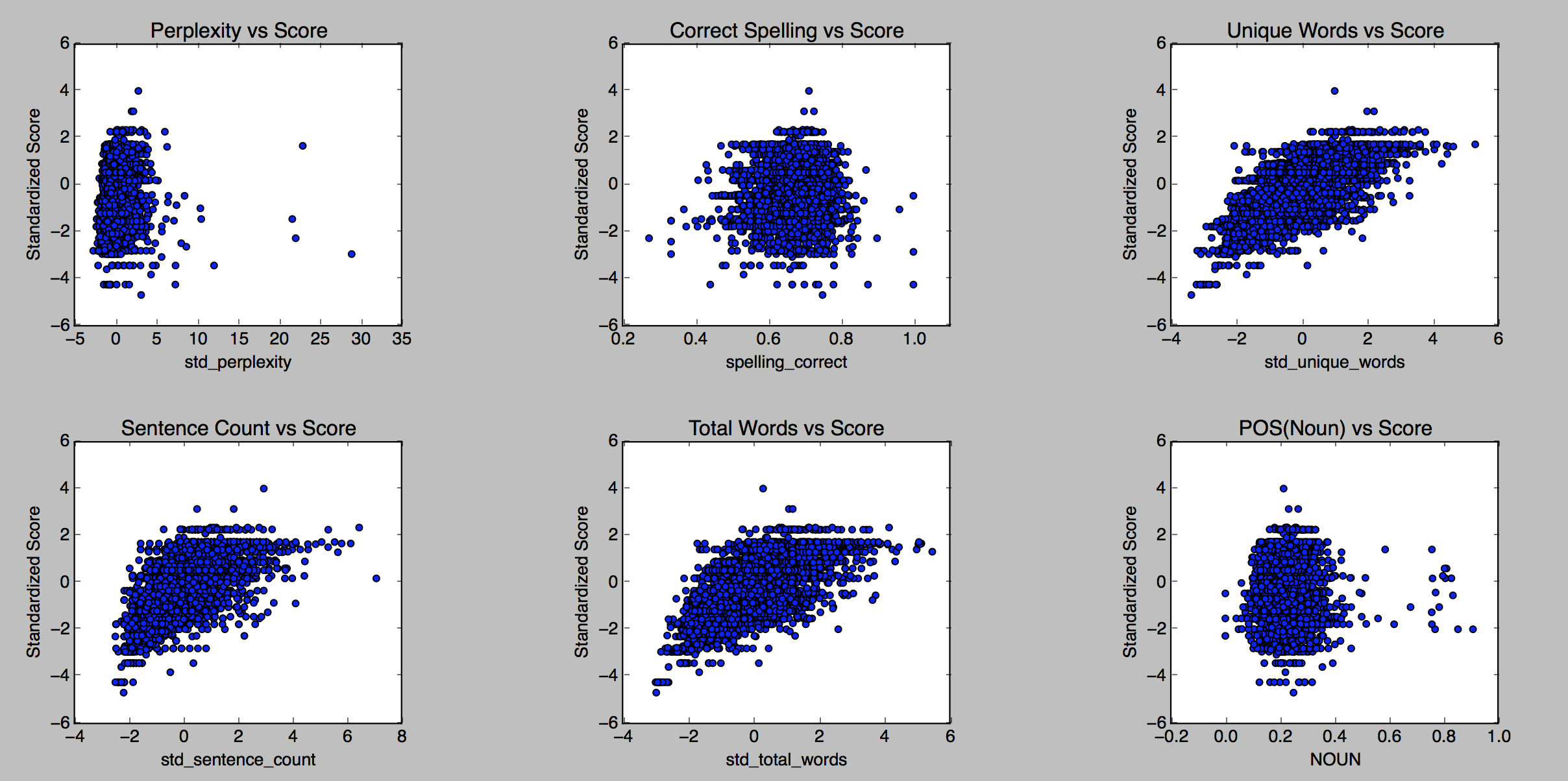
Unique word count, word count, and sentence count all seem to have a clearly correlated relationship with score, while perplexity demonstrates a possible trend. It is our belief that with a more advanced perplexity library, perhaps one based on n-grams rather than unigrams, this relationship would be strengthened. Indeed, this is a point of discussion later in this report.
With these these additional features in place, we moved on to select the actual model to predict our response variable. In the end, we decided to continue using linear regression, as we saw no reason to stray from this approach, and also because we were recommended to use such a model! However, we decided that it was important to include a regularization component in order to limit the influence of any collinear relationships among our thousands of features.
We experimented with both Lasso and Ridge regularization, tuning for optimal alpha with values ranging from 0.05 to 1 in 0.05 increments. As learned in class, Lasso performs both parameter shrinkage and variable selection, automatically removing predictors that are collinear with other predictors. Ridge regression, on the other hand, does not zero out coefficients for the predictors, but does minimize them, limiting their effect on the Spearman correlation.
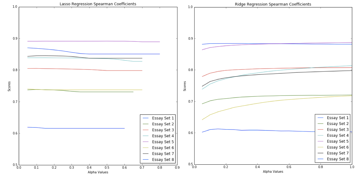
| Set 1 | Set 2 | Set 3 | Set 4 | Set 5 | Set 6 | Set 7 | Set 8 | Average | |
|---|---|---|---|---|---|---|---|---|---|
| Best Alpha | 0.3 | 1 | 1 | 1 | 1 | 1 | 1 | 0.15 | |
| Max Ridge | 0.884028 | 0.720432 | 0.807483 | 0.813519 | 0.887043 | 0.717841 | 0.797747 | 0.612373 | 0.780058 |
| Best Alpha | 0.05 | 0.1 | 0.1 | 0.15 | 0.5 | 0.5 | 0.15 | 0.05 | |
| Max Lasso | 0.870108 | 0.738401 | 0.805037 | 0.838745 | 0.891339 | 0.739961 | 0.84513 | 0.619065 | 0.793473 |
| Linear | 0.780988 | 0.572063 | 0.01791 | 0.590328 | 0.719688 | 0.460429 | 0.611579 | 0.509009 | 0.532749 |
Analysis & Interpretation
With this improved model, we see that the Spearman rank correlations have significantly improved from the baseline model. The Spearman rank correlation values now mostly lie in either the “strong” or “very strong” range, a notable improvement from our baseline model producing mostly “very weak” to “moderate” Spearman values.
In Figure 5, we highlight the scores of the models that yielded the highest Spearman correlations for each of the essay sets. Our highest Spearman correlation was achieved on Essay Set 1, at approximately 0.884, whereas our lowest was achieved on Essay Set 8, at approximately 0.619. It is interesting to note the vast difference in performance across essay sets, a fact that may indicate a failure to sufficiently and successfully generalize the model’s accuracy across such a wide variety of essay sets and prompts. We discuss ways to improve this in the following section.
Figures 4 and 5 also show that Lasso regularization generally performed better than the Ridge regularization, exhibiting better Spearman scores in six out of the eight essay sets; in fact, the average score of Lasso was also slightly higher (.793 as compared to .780). While this difference is not large, we would nonetheless opt for the Lasso model. Given that we have thousands of features with the inclusion of tf-idf, it is likely that plenty of these features are not statistically significant in our linear model. Hence, completely eliminating those features—as Lasso does—rather than just shrinking their coefficients, gives us a more interpretable, computationally efficient, and simpler model.
Ultimately, our Lasso linear regression yielded the greatest overall Spearman correlation, and is intuitively justifiable as a model. With proper tuning for regularization, we note that an alpha value of no greater than 0.5 yielded best results (it should be noted, though, that all nonzero alphas produced comparable Spearman scores, as evidenced in Figure 4). Importantly, p-values remained well below 0.05, confirming the statistical significance of our findings. In layman terms, this high Spearman correlation is significant because it indicates that the scores we have predicted for the essays are relatively similar in rank to the actual scores that the essays have received (as in, if essay A is ranked higher than essay B, our model did well in successfully providing the same conclusion).
Future Work & Concluding Thoughts
In sum, we were able to successfully implement a Lasso linear regression model using both trivial and nontrivial essay features to vastly improve upon our baseline model. While features like word count appear to have the most correlated relationship with score from a graphical standpoint, we believe that a feature such as perplexity, which actually takes a language model into account, would in the long run be a superior predictor. Namely, we would ideally extend our self-implemented perplexity functionality to the n-gram case, rather than simply using unigrams. With this added capability, we believe our model could achieve even greater Spearman correlation scores.
Other features that we believe could improve the effectiveness of the model include parse trees. Parse trees are ordered trees that represent the syntactic structure of a phrase. This linguistic model is, much like perplexity, based on content rather than the “metadata” that many trivial features provide. As such, it may prove effective in contributing to the model a more in-depth analysis of the context and construction of sentences, pointing to writing styles that may correlate to higher grades. Finally, we would like to take the prompts of the essays into account. This could be a significant feature for our model, because depending on the type of essay being writing—e.g. persuasive, narrative, summary—the organization of the essay could vary, which would then affect how we create our models and which features become more important.
There is certainly room for improvement on our model—namely, the features we just mentioned, as well as many more we have not discussed. However, given the time, resources and scope for this project, we were very pleased with our results. None of us had ever performed NLP before, but we now look forward to continuing to apply statistical methodology to such problems in the future!
References
- U.S. Bureau of Labor Statistics. "What High School Teachers Do." U.S. Bureau of Labor Statistics, Dec. 2015. Web. 13 Dec. 2016. http://www.bls.gov/ooh/education-training-and-library/high-school-teachers.htm#tab-2.
- The Hewlett Foundation. "The Hewlett Foundation: Automated Essay Scoring." Kaggle, Feb. 2012. Web. 13 Dec. 2016. https://www.kaggle.com/c/asap-aes.
- "Spearman's Correlation." Statstutor, n.d. Web. 14 Dec. 2016. http://www.statstutor.ac.uk/resources/uploaded/spearmans.pdf
- Berwick, Robert C. "Natural Language Processing Notes for Lectures 2 and 3, Fall 2012." Massachusetts Institute of Technology - Natural Language Processing Course. Massachusetts Institute of Technology, n.d. Web. 13 Dec. 2016. http://web.mit.edu/6.863/www/fall2012/lectures/lecture2&3-notes12.pdf.
- "NgramModel No Longer Available? - Issue #738 - Nltk/nltk." GitHub. NLTK Open Source Library, Aug. 2014. Web. 13 Dec. 2016. https://github.com/nltk/nltk/issues/738.